Tancik et al. [1] recently performed a series of interesting experiments showing that positional encoding with random Fourier features (RFFs) significantly improves learning of high-frequency details on various tasks in computer graphics and image processing (e.g., image regression, shape representation, MRI reconstruction and inverse rendering). Their results are nicely illustrated in this figure (alse see https://github.com/tancik/fourier-feature-networks).
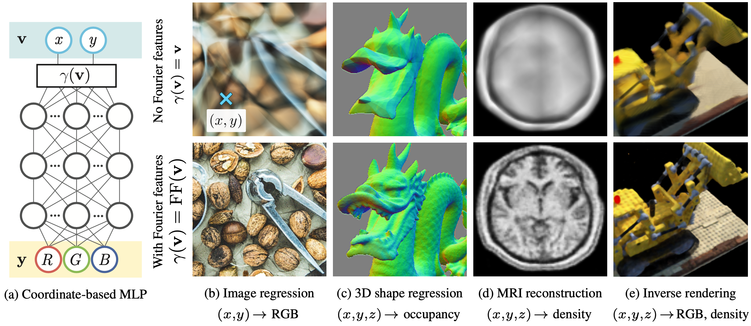
Given the strong properties of RFFs, let us investigate if these can be combined with pattern-producing networks and trees to generate interesting abstract graphics.
Random Fourier features (RFFs)
RFFs were originally introduced by Rahimi and Recht [2] for kernel approximation. For our purposes, we define these features as:
\[\text{RFF}(\mathbf{v})= \left( \cos(2\pi\mathbf{f}_1^T\mathbf{v}), \sin(2\pi\mathbf{f}_1^T\mathbf{v}), \cos(2\pi\mathbf{f}_2^T\mathbf{v}), \sin(2\pi\mathbf{f}_2^T\mathbf{v}), \ldots, \cos(2\pi\mathbf{f}_N^T\mathbf{v}), \sin(2\pi\mathbf{f}_N^T\mathbf{v}) \right)^T\]where $\mathbf{v}$ is the input vector to be transformed and there are $N$ frequency vectors $\mathbf{f}_1, \mathbf{f}_2, \ldots, \mathbf{f}_N$.
Each of these frequency vectors is sampled from a normal distribution with a zero mean and a diagonal covariance matrix of the form $\sigma^2\mathbf{I}$.
The standard deviation $\sigma$ is the most interesting property of the encoding as it sets the level of detail that can be represented.
Positional encoding and generative graphics
Recall that CPPNs are nothing else than multilayer perceptrons (MLPs) with random weights that map an $(x, y)$ position into an RGB color value for that position:
However, let us transform $\mathbf{v}=(x, y)^T$ before it goes into the MLP:
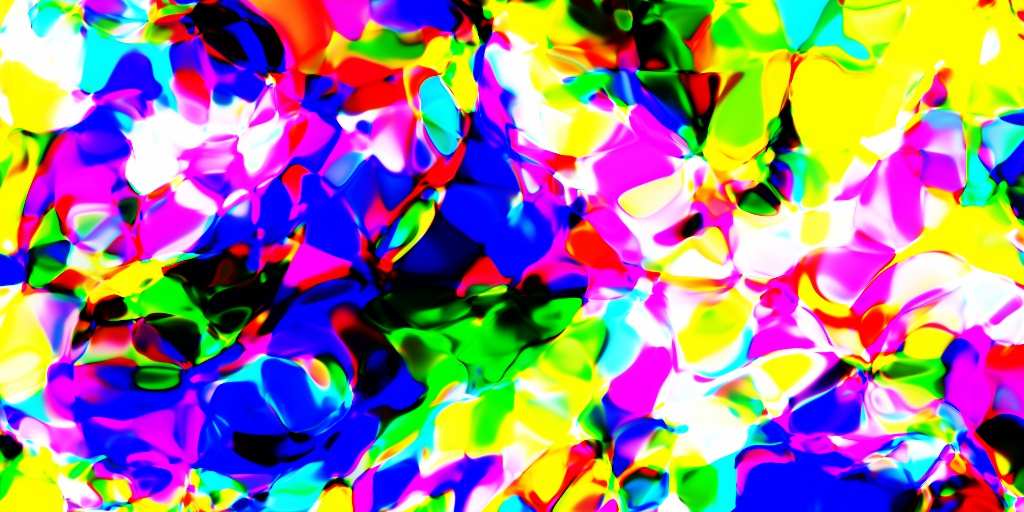
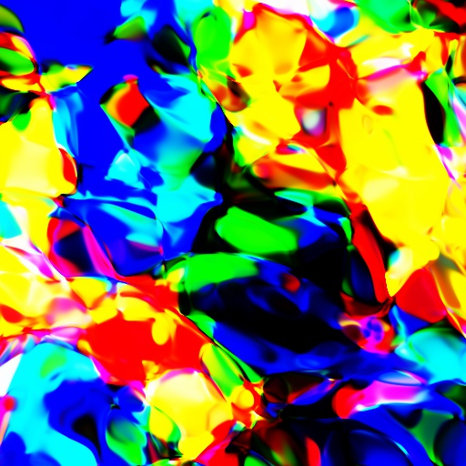
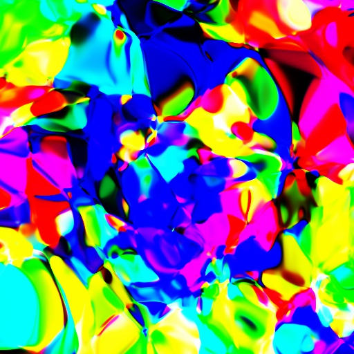
The produced visual patterns are interesting and qualitatively different than the ones in our previous CPPN post:
The script imggen-cppn.py enables you to produce similar patterns for varying standard deviation $\sigma$.
python3 imggen-cppn.py 2.0 out.jpg
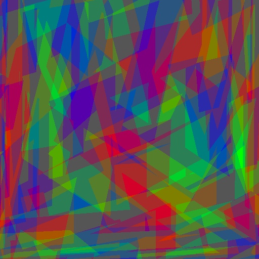
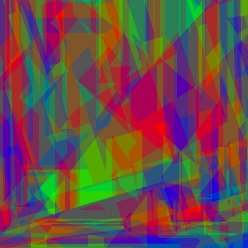
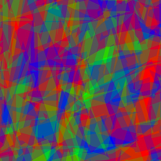
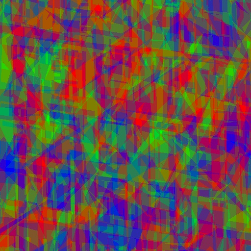
Here are four examples for $\sigma=1, 2, 3, 4$:
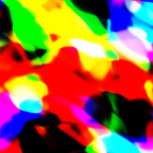
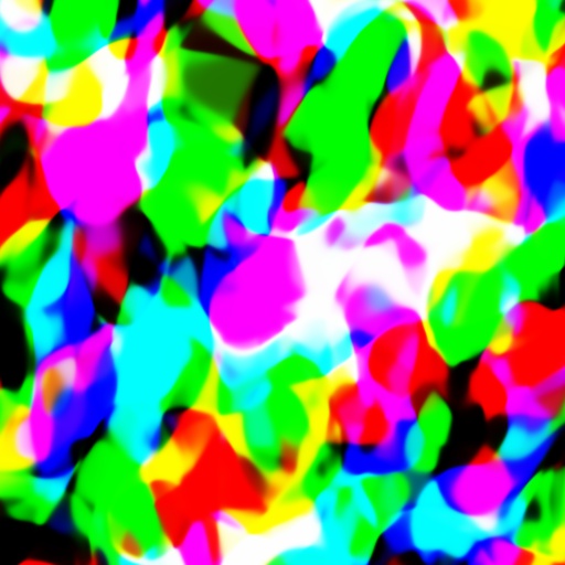
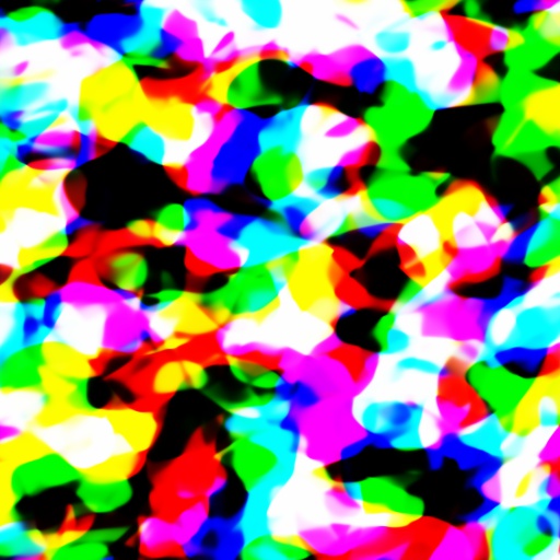
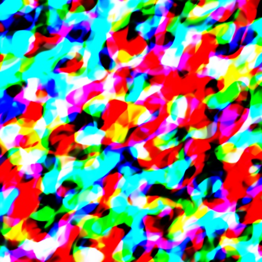
We can observe that the amount of color mixing and spatial details steadily increases with $\sigma$.
We can also add a temporal dimension to produce videos such as the following one (code):
Pattern-producing trees
Instead of an MLP, we can use randomized trees. The code for this experiment is available here. We can invoke it as follows:
python3 imggen-ppts.py 2.0 out.jpg
Here are some examples for varying standard deviation:
Resources
[1] Tancik et al. Fourier Features Let Networks Learn High Frequency Functions in Low Dimensional Domains. https://arxiv.org/abs/2006.10739, 2020
[2] Ali Rahimi and Ben Recht. Random Features for Large-Scale Kernel Machines. NIPS, 2007