Some experiments in learning signed distance fields from data

There has been considerable interest in learning-based methods for signed distance field modeling. And this is lately especially true in the area of deep learning: see section “Implicit representation” at https://github.com/subeeshvasu/Awsome_Deep_Geometry_Learning.

Thus, it is warranted to investigate whether gridhopping and LambdaCAD are useful in this area. E.g., for extracting polygonal models from such representations for debugging or rendering purposes.

References [1, 2, 3, 4] are a selection of interesting papers on geometric deep learning. These papers illustrate some core ideas and applications within the area. The first two study the learning of generative models for 3D shapes. I.e., for applications that need to generate novel 3D shapes belonging to a certain class, such as aeroplanes of cars. This could be useful in computer games and some types of viritual reality software, for example. In [1], the authors propose to model a shape as an occupancy map (\(+1\) outside shape, \(-1\) inside) with a neural network classifier. Since this representaion is smooth, it is capable of defining shapes as implicit sufraces. However, the approach would probably not work well with sphere tracing because of issues ontlined in a previous post about Lipschitz continuity. On the other hand, the authors of [2] propose to model a 3D shape \(S\) with a neural network that is learned to estimate the signed distance field:

Of course, there are some caveats that simplify the process and enable learning of a generative model. Please see the paper for these details. Even though the network is explicitly learned to approximate the distance to the shape, there is no guarantee that sphere tracing will work as intended (especially when far away from the shape), but we expect less problems than with occupancy maps. The paper by Li et al. [3] contains a similar approach to that of [2] except that it is not concerned with generative modeling, but with shape compression. I.e., each shape is assigned a separate tiny network that approximates its signed distance field. The hope is that this tiny network requires less memory to store than an explicit list of polygons, effectively enabling a compressed representation. Thus, this approach has the same potential to be compatible with gridhopping as [2]. The fourth paper mentioned earlier (Davies et al. [4]) uses a neural network that outputs a list of primitives and their parameters to approximate an input point cloud. Since the basic primitives used (spheres, cones, etc.) have explicit and efficiently computable signed distance fields, this approach is compatible with gridhopping.

Given the interesting resluts presented in the mentioned papers, we experiment with two learning algorithms for converting a 3D polygonal mesh into a signed distance field. The first one is based on random Fourier features and the second one on a simple feedforward neural network. However, let us first describe the shapes we use and how we prepare the training data.

Training data

We use the following 3D shapes:

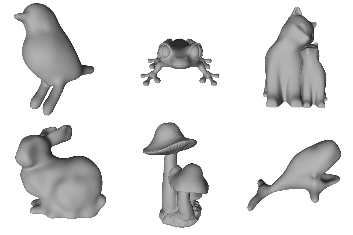
These were downloaded from the Thingi10K dataset. See reference [5] for more details.

Our goal is to transform these shapes into signed distance fields.

Given such a shape \(S\), we generate a trainig set of the form

where \(\mathbf{x}\in\mathbb{R}^3\) is a point in 3D space and \(d_i\) is the Euclidean distance from \(\mathbf{x}\) to the surface of \(S\). This is conceptually very simple, but there are some subtleties.

In our experiments, \(S\) is represented as a triangle mesh. We generate the trainig data with the help of the excellent mesh-to-sdf library:

import mesh_to_sdf
import trimesh
mesh = trimesh.load("/path/to/mesh.stl")
xyz, dists = mesh_to_sdf.sample_sdf_near_surface(mesh, number_of_points=250000)
xyz, dists = xyz/2.0, dists/2.0 # normalize to unit cube

After the above code is executed, the xyz variable is a 2D numpy array containing \(250\;000\) \((x, y, z)\) points sampled inside a unit cube centered at the origin and dists contains the distances of these points to the shape. Some of the points are sampled uniformly inside the unit cube, but the majority come from the surface of the mesh. Of course, prior to sampling, the mesh is re-scaled to fit the unit cube. An example point cloud obtained in this way is illustrated in the following image:

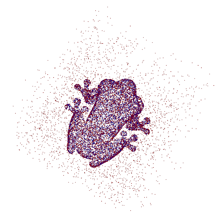
The points outside the shape are colorized red and the ones inside are blue. These inside points are assigned negative distances. This is the usual procedure when working with signed distance fields.

Given such a training set, we can now describe two basic learning approaches that are used in our gridhopping experiments later.

Approximating a signed distance field with weighted Fourier features

We have used Fourier features in a previous post, but we go over the basics here once again for completeness.

Let \(\mathbf{v}=(x, y, z)^T\) be a vector representing a point location in 3D space. Fourier features computed from \(\mathbf{v}\) are defined as

where \(\mathbf{f}_i\) are the frequency vectors. In our experiments, we sample these from a standard normal distribusion with zero mean and a standard deviation \(\sigma\). Of course, \(\mathbf{f}_i\)s are generated at the beginning and stay fixed during the whole experiment. Setting \(\sigma=3\), \(N=1024\) worked well for in our experiments and thus we keep these values.

The idea is to approximate the signed distance \(d_S\) to shape \(S\) as a weighted average of Fourier features:

The weights \(\mathbf{w}\in\mathbb{R}^{2N}\) have to be computed (learned) with some kind of an optimization procedure. A simple and effective procedure is to first compute Fourier features for all poitns \(\mathbf{v}_j\) in the dataset:

and then find \(\mathbf{w}\) that minimizes

where \(d_j=d_S(\mathbf{v}_j)\) is the distance from the \(j\)th point to the shape \(S\).

This is an ordinary least squares problem and it has an efficient closed-form solution: https://en.wikipedia.org/wiki/Ordinary_least_squares. These properties make the proposed method quite elegant. However, we have encountered several empirical shortcomings when dealing with more complex shapes. Detailed analysis of these issues is out of scope for this post and we now focus on gridhopping.

You may recall that if certain criteria are not met, gridhopping might “miss” parts of the surface of the shape and render an incomplete mesh. To circumvent these problems, we shrink the signed distance approximation by factor \(\lambda\):

Note that using a too large \(\lambda\) reduces the efficiency of gridhopping, i.e., more SDF evaluations are needed to localize the grid cells containing the shape surface. Thus, we want the smallest possible value that results in correct polygonization. We empirically found that setting \(\lambda=1.5\) works well. It is important to say that this does not affect the final mesh. I.e., the meshes computed by gridhopping and the basic algorithm of cubic complexity are the same. The only difference should be in speed. We check this hypothesis next.

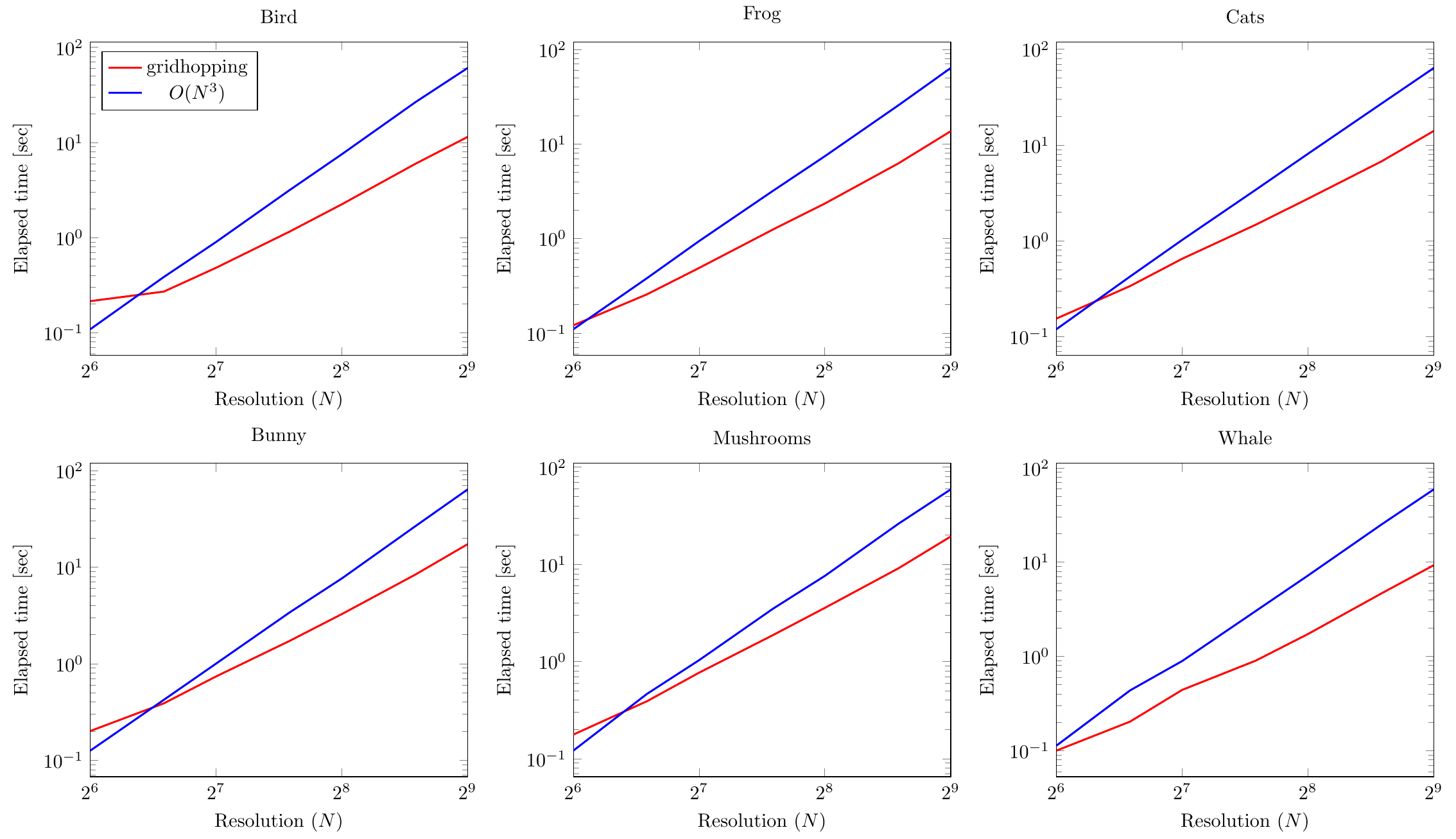
We compare times needed to polygonize SDFs of our 6 learned models for the basic \(O(N^3)\) algorithm and gridhopping. The grid resolution \(N\) varies from \(64\) to \(512\). The basic method should scale as \(O(N^3)\) and gridhopping as \(O(N^2\log N)\) (see here for a theoretical analysis that produces this). Batching the SDF evaluations in chunks of size \(\approx 10\;000\) leads to speed improvements. All computations are performed on a relatively high-end laptop CPU: Intel(R) Core(TM) i7-9750H CPU @ 2.60GHz. The results can be seen in the figures below (the legend for all is in the top left one):

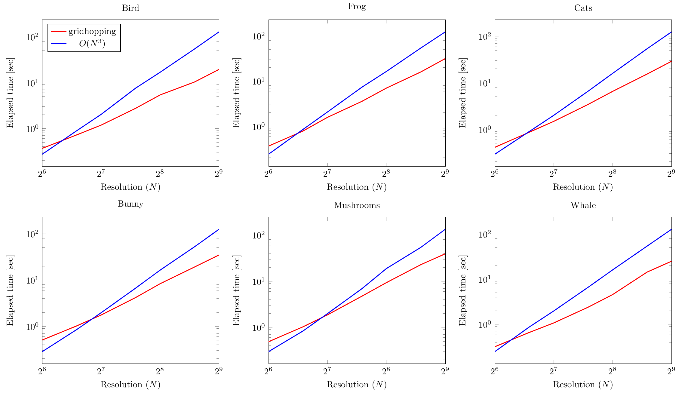
First of all, note that both the abscissae and ordinates are logarithmic. We can see that all timing plots appear as lines in the figures. And if you analyze their slopes, it indeed empirically verifies the theoretically predicted computational complexities. This confirms our theory that gridhopping is significantly asymptotically faster than the basic algorithm.

Let us check next how all this works when we represent the SDF with a neural network instead.

Approximating a signed distance field with neural networks

The basic idea is to train a neural network NN with paramters \(\theta\) that transforms the input \(\mathbf{v}=(x, y, z)^T\) coordinates into a distance to the shape \(S\):

We use a simple network architecture in our experiments. It is not excluded that better results (more accuracy, speed improvement, etc.) would be achieved by spending more time on its design. Following Davies et al. [4], our networks have a feedforward fully-connected architecture with 8 layers. Each layer has a hidden size of 64 and the activation function is set to be a ReLU. To speed up training, we also use batch normalization in all layers except the last one. This results in about \(30000\) network parameters (120kB of memory). By modern standards, this is a tiny network, but it is capable of accurately representing the shapes used in our experiments.

The networks are learned with the standard stochastic gradient descent approach. We use the Adam optimizer [6] with the learning rate set to \(0.0001\). The gradient-related updates are computed on minibatches containing \(512\) point-distance pairs. The total number of updates is limited to \(200\;000\) and thus the GPU-accelerated training finishes in less than one hour for each network. These settings seem to generalize well across a wide range of geometries.

The following NN evaluations are performed on an Nvidia GeForce RTX 2060 Mobile GPU. It is important to note that we noticed a significant relation between processing speed and batching size, i.e., how much points/rays we process in parallel. It seems that the optimal value is around \(100\;000\) for the mentioned hardware setup. The results can be seen in the figures below (the legend for all is in the top left one):

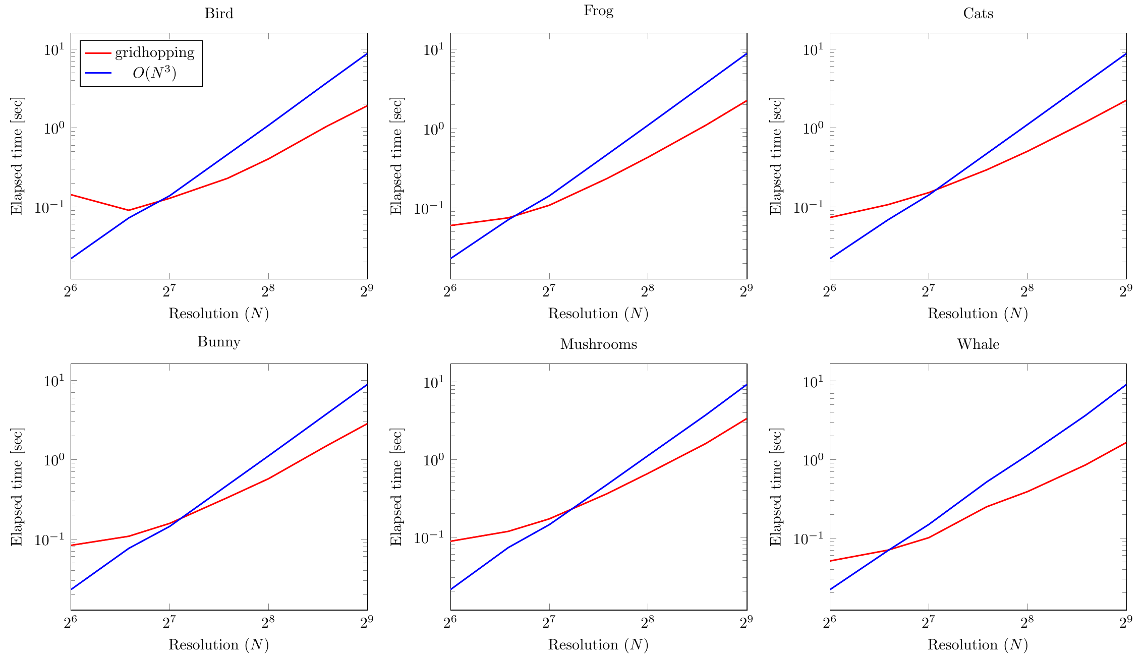
Since the axes are logarithmic again, we can observe that gridhopping is asymptotically better (something like \(O(N^2)\)) than the basic \(O(N^3)\) method. However, for values of grid resolution \(N\) smaller than about \(2^7=128\), the basic method is faster. We attribute this fact to constant overhead needed to prepare the gridhopping run.

For completeness of our exposition, we also repeat all computations on a laptop CPU (same setup as in FF experiments). The results can be seen in figures below:

We observe a similar asymptotical trend (for large values of \(N\)): gridhopping has a computational complexity advantage over the basic method. It can even be seen that for some models the advantage holds even for smaller grid resolutions.

Conclusion

We have experimentally shown that the gridhopping method has a significant computational benefit for polygonizing signed distance functions that are learned from data. This result could prove useful for computer games and virtual world software where compressed representations [4] are required for storage reasons. Another interesting application is sampling from parametric distributions [2] followed by polygonization for achieving greater model/world variety.

The source code for our experiments is available at https://github.com/nenadmarkus/gridhopping:

• FF experiments
• NN experiments

The learned NN models can be downloaded here.

References

[1] Zhiqin Chen and Hao Zhang. Learning Implicit Fields for Generative Shape Modeling. CVPR, 2019 (arXiv)

[2] Park et al. DeepSDF: Learning Continuous Signed Distance Functionsfor Shape Representation. CVPR, 2019 (arXiv)

[3] Li et al. Supervised Fitting of Geometric Primitives to 3D Point Clouds. CVPR, 2019 (arXiv)

[4] Davies et al. Overfit Neural Networks as a Compact Shape Representation. https://arxiv.org/abs/2009.09808, 2020

[5] Qingnan Zhou and Alec Jacobson. Thingi10K: A Dataset of 10,000 3D-Printing Models. https://arxiv.org/abs/1605.04797, 2016

[6] Diederik P. Kingma and Jimmy Ba. Adam: A Method for Stochastic Optimization. ICLR, 2015 (arXiv)